Importing Data in the Tidyverse
Data are stored in all sorts of different file formats and structures. In this course, we'll discuss each of these common formats and discuss how to get them into R so you can start working with them!
About This Course
Getting data into your statistical analysis system can be one of the most challenging parts of any data science project. Data must be imported and harmonized into a coherent format before any insights can be obtained. You will learn how to get data into R from commonly used formats and how to harmonize different kinds of datasets from different sources. If you work in an organization where different departments collect data using different systems and different storage formats, then this course will provide essential tools for bringing those datasets together and making sense of the wealth of information in your organization.
This course introduces the Tidyverse tools for importing data into R so that it can be prepared for analysis, visualization, and modeling. Common data formats are introduced, including delimited files, spreadsheets, and relational databases. We will also introduce techniques for obtaining data from the web, such as web scraping and getting data from web APIs.
In this specialization we assume familiarity with the R programming language. If you are not yet familiar with R, we suggest you first complete R Programming before returning to complete this course.
Tibbles
Before we can discuss any particular file format, let's discuss the end goal - the tibble! If you've been using R for a while, you're likely familiar with the data.frame. It's best to think of tibbles as an updated and stylish version of the data.frame. And, tibbles are what tidyverse packages work with most seamlessly. Now, that doesn't mean tidyverse packages require tibbles. In fact, they still work with data.frames, but the more you work with tidyverse and tidyverse-adjacent packages, the more you'll see the advantages of using tibbles.
Before we go any further, tibbles are data frames, but they have some new bells and whistles to make your life easier.
How tibbles differ from data.frame
There are a number of differences between tibbles and data.frames. To see a full vignette about tibbles and how they differ from data.frame, you'll want to execute vignette('tibble') and read through that vignette. However, we'll summarize some of the most important points here:
- Input type remains unchanged - data.frame is notorious for treating strings as factors; this will not happen with tibbles
- Variable names remain unchanged - In base R, creating data.frames will remove spaces from names, converting them to periods or add 'x' before numeric column names. Creating tibbles will not change variable (column) names.
- There are no
row.names()for a tibble - Tidy data requires that variables be stored in a consistent way, removing the need for row names. - Tibbles print first ten rows and columns that fit on one screen - Printing a tibble to screen will never print the entire huge data frame out. By default, it just shows what fits to your screen.
Creating a tibble
The tibble package is part of the tidyverse and can thus be loaded in (once installed) using:
as_tibble()
Since many packages use the historical data.frame from base R, you'll often find yourself in the situation that you have a data.frame and want to convert that data.frame to a tibble. To do so, the as_tibble() function is exactly what you're looking for.
For example, the trees dataset is a data.frame that's available in base R. This dataset stores the diameter, height, and volume for Black Cherry Trees. To convert this data.frame to a tibble you would use the following:
## # A tibble: 31 × 3 ## Girth Height Volume ## <dbl> <dbl> <dbl> ## 1 8.3 70 10.3 ## 2 8.6 65 10.3 ## 3 8.8 63 10.2 ## 4 10.5 72 16.4 ## 5 10.7 81 18.8 ## 6 10.8 83 19.7 ## 7 11 66 15.6 ## 8 11 75 18.2 ## 9 11.1 80 22.6 ## 10 11.2 75 19.9 ## # … with 21 more rows Note in the above example and as mentioned earlier, that tibbles, by default, only print the first ten rows to screen. If you were to print trees to screen, all 31 rows would be displayed. When working with large data.frames, this default behavior can be incredibly frustrating. Using tibbles removes this frustration because of the default settings for tibble printing.
Additionally, you'll note that the type of the variable is printed for each variable in the tibble. This helpful feature is another added bonus of tibbles relative to data.frame.
If you do want to see more rows from the tibble, there are a few options! First, the View() function in RStudio is incredibly helpful. The input to this function is the data.frame or tibble you'd like to see. Specifically, View(trees) would provide you, the viewer, with a scrollable view (in a new tab) of the complete dataset.
A second option is the fact that print() enables you to specify how many rows and columns you'd like to display. Here, we again display the trees data.frame as a tibble but specify that we'd only like to see 5 rows. The width = Inf argument specifies that we'd like to see all the possible columns. Here, there are only 3, but for larger datasets, this can be helpful to specify.
as_tibble(trees) %>% print(n = 5, width = Inf) ## # A tibble: 31 × 3 ## Girth Height Volume ## <dbl> <dbl> <dbl> ## 1 8.3 70 10.3 ## 2 8.6 65 10.3 ## 3 8.8 63 10.2 ## 4 10.5 72 16.4 ## 5 10.7 81 18.8 ## # … with 26 more rows Other options for viewing your tibbles are the slice_* functions of the dplyr package.
The slice_sample() function of the dplyr package will allow you to see a sample of random rows in random order. The number of rows to show is specified by the n argument. This can be useful if you don't want to print the entire tibble, but you want to get a greater sense of the values. This is a good option for data analysis reports, where printing the entire tibble would not be appropriate if the tibble is quite large.
slice_sample(trees, n = 10) ## Girth Height Volume ## 1 16.3 77 42.6 ## 2 14.0 78 34.5 ## 3 13.8 64 24.9 ## 4 10.8 83 19.7 ## 5 8.8 63 10.2 ## 6 17.5 82 55.7 ## 7 8.3 70 10.3 ## 8 11.4 76 21.4 ## 9 10.7 81 18.8 ## 10 10.5 72 16.4 You can also use slice_head() or slice_tail() to take a look at the top rows or bottom rows of your tibble. Again the number of rows can be specified with the n argument.
This will show the first 5 rows.
## Girth Height Volume ## 1 8.3 70 10.3 ## 2 8.6 65 10.3 ## 3 8.8 63 10.2 ## 4 10.5 72 16.4 ## 5 10.7 81 18.8 This will show the last 5 rows.
## Girth Height Volume ## 1 17.5 82 55.7 ## 2 17.9 80 58.3 ## 3 18.0 80 51.5 ## 4 18.0 80 51.0 ## 5 20.6 87 77.0 tibble()
Alternatively, you can create a tibble on the fly by using tibble() and specifying the information you'd like stored in each column. Note that if you provide a single value, this value will be repeated across all rows of the tibble. This is referred to as 'recycling inputs of length 1.'
In the example here, we see that the column c will contain the value '1' across all rows.
tibble( a = 1 : 5, b = 6 : 10, c = 1, z = (a + b)^ 2 + c ) ## # A tibble: 5 × 4 ## a b c z ## <int> <int> <dbl> <dbl> ## 1 1 6 1 50 ## 2 2 7 1 82 ## 3 3 8 1 122 ## 4 4 9 1 170 ## 5 5 10 1 226 The tibble() function allows you to quickly generate tibbles and even allows you to reference columns within the tibble you're creating, as seen in column z of the example above.
We also noted previously that tibbles can have column names that are not allowed in data.frame. In this example, we see that to utilize a nontraditional variable name, you surround the column name with backticks. Note that to refer to such columns in other tidyverse packages, you'll continue to use backticks surrounding the variable name.
tibble( ` two words ` = 1 : 5, ` 12 ` = 'numeric', ` :) ` = 'smile', ) ## # A tibble: 5 × 3 ## `two words` `12` `:)` ## <int> <chr> <chr> ## 1 1 numeric smile ## 2 2 numeric smile ## 3 3 numeric smile ## 4 4 numeric smile ## 5 5 numeric smile Subsetting
Subsetting tibbles also differs slightly from how subsetting occurs with data.frame. When it comes to tibbles, [[ can subset by name or position; $ only subsets by name. For example:
df <- tibble( a = 1 : 5, b = 6 : 10, c = 1, z = (a + b)^ 2 + c ) # Extract by name using $ or [[]] df$z ## [1] 50 82 122 170 226 ## [1] 50 82 122 170 226 # Extract by position requires [[]] df[[4]] ## [1] 50 82 122 170 226 Having now discussed tibbles, which are the type of object most tidyverse and tidyverse-adjacent packages work best with, we now know the goal. In many cases, tibbles are ultimately what we want to work with in R. However, data are stored in many different formats outside of R. We'll spend the rest of this course discussing those formats and talking about how to get those data into R so that you can start the process of working with and analyzing these data in R.
Spreadsheets
Spreadsheets are an incredibly common format in which data are stored. If you've ever worked in Microsoft Excel or Google Sheets, you've worked with spreadsheets. By definition, spreadsheets require that information be stored in a grid utilizing rows and columns.
Excel files
Microsoft Excel files, which typically have the file extension .xls or .xlsx, store information in a workbook. Each workbook is made up of one or more spreadsheet. Within these spreadsheets, information is stored in the format of values and formatting (colors, conditional formatting, font size, etc.). While this may be a format you've worked with before and are familiar, we note that Excel files can only be viewed in specific pieces of software (like Microsoft Excel), and thus are generally less flexible than many of the other formats we'll discuss in this course. Additionally, Excel has certain defaults that make working with Excel data difficult outside of Excel. For example, Excel has a habit of aggressively changing data types. For example if you type 1/2, to mean 0.5 or one-half, Excel assumes that this is a date and converts this information to January 2nd. If you are unfamiliar with these defaults, your spreadsheet can sometimes store information other than what you or whoever entered the data into the Excel spreadsheet may have intended. Thus, it's important to understand the quirks of how Excel handles data. Nevertheless, many people do save their data in Excel, so it's important to know how to work with them in R.
Reading Excel files into R
Reading spreadsheets from Excel into R is made possible thanks to the readxl package. This is not a core tidyverse package, so you'll need to install and load the package in before use:
##install.packages('readxl') library(readxl) The function read_excel() is particularly helpful whenever you want read an Excel file into your R Environment. The only required argument of this function is the path to the Excel file on your computer. In the following example, read_excel() would look for the file 'filename.xlsx' in your current working directory. If the file were located somewhere else on your computer, you would have to provide the path to that file.
# read Excel file into R df_excel <- read_excel('filename.xlsx') Within the readxl package there are a number of example datasets that we can use to demonstrate the packages functionality. To read the example dataset in, we'll use the readxl_example() function.
# read example file into R example <- readxl_example('datasets.xlsx') df <- read_excel(example) df ## # A tibble: 150 × 5 ## Sepal.Length Sepal.Width Petal.Length Petal.Width Species ## <dbl> <dbl> <dbl> <dbl> <chr> ## 1 5.1 3.5 1.4 0.2 setosa ## 2 4.9 3 1.4 0.2 setosa ## 3 4.7 3.2 1.3 0.2 setosa ## 4 4.6 3.1 1.5 0.2 setosa ## 5 5 3.6 1.4 0.2 setosa ## 6 5.4 3.9 1.7 0.4 setosa ## 7 4.6 3.4 1.4 0.3 setosa ## 8 5 3.4 1.5 0.2 setosa ## 9 4.4 2.9 1.4 0.2 setosa ## 10 4.9 3.1 1.5 0.1 setosa ## # … with 140 more rows Note that the information stored in df is a tibble. This will be a common theme throughout the packages used in these courses.
Further, by default, read_excel() converts blank cells to missing data (NA). This behavior can be changed by specifying the na argument within this function. There are a number of additional helpful arguments within this function. They can all be seen using ?read_excel, but we'll highlight a few here:
-
sheet- argument specifies the name of the sheet from the workbook you'd like to read in (string) or the integer of the sheet from the workbook. -
col_names- specifies whether the first row of the spreadsheet should be used as column names (default: TRUE). Additionally, if a character vector is passed, this will rename the columns explicitly at time of import. -
skip- specifies the number of rows to skip before reading information from the file into R. Often blank rows or information about the data are stored at the top of the spreadsheet that you want R to ignore.
For example, we are able to change the column names directly by passing a character string to the col_names argument:
# specify column names on import read_excel(example, col_names = LETTERS[1 : 5]) ## # A tibble: 151 × 5 ## A B C D E ## <chr> <chr> <chr> <chr> <chr> ## 1 Sepal.Length Sepal.Width Petal.Length Petal.Width Species ## 2 5.1 3.5 1.4 0.2 setosa ## 3 4.9 3 1.4 0.2 setosa ## 4 4.7 3.2 1.3 0.2 setosa ## 5 4.6 3.1 1.5 0.2 setosa ## 6 5 3.6 1.4 0.2 setosa ## 7 5.4 3.9 1.7 0.4 setosa ## 8 4.6 3.4 1.4 0.3 setosa ## 9 5 3.4 1.5 0.2 setosa ## 10 4.4 2.9 1.4 0.2 setosa ## # … with 141 more rows To take this a step further let's discuss one of the lesser-known arguments of the read_excel() function: .name_repair. This argument allows for further fine-tuning and handling of column names.
The default for this argument is .name_repair = 'unique'. This checks to make sure that each column of the imported file has a unique name. If TRUE, readxl leaves them as is, as you see in the example here:
# read example file into R using .name_repair default read_excel( readxl_example('deaths.xlsx'), range = 'arts!A5:F8', .name_repair = 'unique' ) ## # A tibble: 3 × 6 ## Name Profession Age `Has kids` `Date of birth` `Date of death` ## <chr> <chr> <dbl> <lgl> <dttm> <dttm> ## 1 David Bowie musician 69 TRUE 1947-01-08 00:00:00 2016-01-10 00:00:00 ## 2 Carrie Fisher actor 60 TRUE 1956-10-21 00:00:00 2016-12-27 00:00:00 ## 3 Chuck Berry musician 90 TRUE 1926-10-18 00:00:00 2017-03-18 00:00:00 Another option for this argument is .name_repair = 'universal'. This ensures that column names don't contain any forbidden characters or reserved words. It's often a good idea to use this option if you plan to use these data with other packages downstream. This ensures that all the column names will work, regardless of the R package being used.
# require use of universal naming conventions read_excel( readxl_example('deaths.xlsx'), range = 'arts!A5:F8', .name_repair = 'universal' ) ## New names: ## * `Has kids` -> Has.kids ## * `Date of birth` -> Date.of.birth ## * `Date of death` -> Date.of.death ## # A tibble: 3 × 6 ## Name Profession Age Has.kids Date.of.birth Date.of.death ## <chr> <chr> <dbl> <lgl> <dttm> <dttm> ## 1 David Bowie musician 69 TRUE 1947-01-08 00:00:00 2016-01-10 00:00:00 ## 2 Carrie Fisher actor 60 TRUE 1956-10-21 00:00:00 2016-12-27 00:00:00 ## 3 Chuck Berry musician 90 TRUE 1926-10-18 00:00:00 2017-03-18 00:00:00 Note that when using .name_repair = 'universal', you'll get a readout about which column names have been changed. Here you see that column names with a space in them have been changed to periods for word separation.
Aside from these options, functions can be passed to .name_repair. For example, if you want all of your column names to be uppercase, you would use the following:
# pass function for column naming read_excel( readxl_example('deaths.xlsx'), range = 'arts!A5:F8', .name_repair = toupper ) ## # A tibble: 3 × 6 ## NAME PROFESSION AGE `HAS KIDS` `DATE OF BIRTH` `DATE OF DEATH` ## <chr> <chr> <dbl> <lgl> <dttm> <dttm> ## 1 David Bowie musician 69 TRUE 1947-01-08 00:00:00 2016-01-10 00:00:00 ## 2 Carrie Fisher actor 60 TRUE 1956-10-21 00:00:00 2016-12-27 00:00:00 ## 3 Chuck Berry musician 90 TRUE 1926-10-18 00:00:00 2017-03-18 00:00:00 Notice that the function is passed directly to the argument. It does not have quotes around it, as we want this to be interpreted as the toupper() function.
Here we've really only focused on a single function (read_excel()) from the readxl package. This is because some of the best packages do a single thing and do that single thing well. The readxl package has a single, slick function that covers most of what you'll need when reading in files from Excel. That is not to say that the package doesn't have other useful functions (it does!), but this function will cover your needs most of the time.
Google Sheets
Similar to Microsoft Excel, Google Sheets is another place in which spreadsheet information is stored. Google Sheets also stores information in spreadsheets within workbooks. Like Excel, it allows for cell formatting and has defaults during data entry that could get you into trouble if you're not familiar with the program.
Unlike Excel files, however, Google Sheets live on the Internet, rather than your computer. This makes sharing and updating Google Sheets among people working on the same project much quicker. This also makes the process for reading them into R slightly different. Accordingly, it requires the use of a different, but also very helpful package, googlesheets4!
As Google Sheets are stored on the Internet and not on your computer, the googlesheets4 package does not require you to download the file to your computer before reading it into R. Instead, it reads the data into R directly from Google Sheets. Note that if the data hosted on Google Sheets changes, every time the file is read into R, the most updated version of the file will be utilized. This can be very helpful if you're collecting data over time; however, it could lead to unexpected changes in results if you're not aware that the data in the Google Sheet is changing.
To see exactly what we mean, let's look at a specific example. Imagine you've sent out a survey to your friends asking about how they spend their day. Let's say you're mostly interested in knowing the hours spent on work, leisure, sleep, eating, socializing, and other activities. So in your Google Sheet you add these six items as columns and one column asking for your friends names. To collect this data, you then share the link with your friends, giving them the ability to edit the Google Sheet.
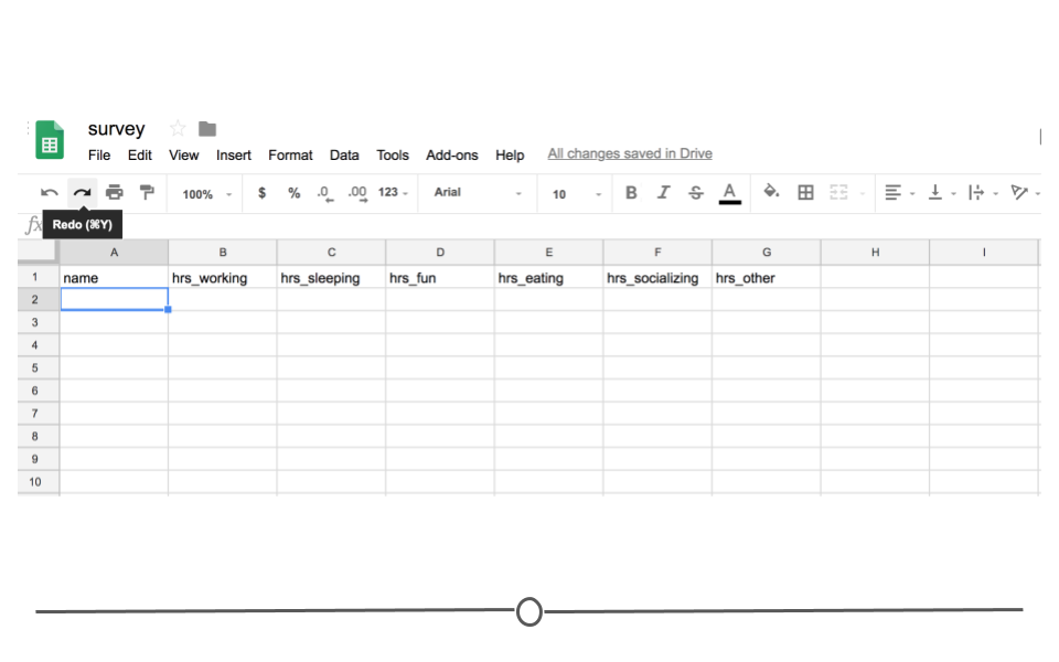
Survey Google Sheets
Your friends will then one-by-one complete the survey. And, because it's a Google Sheet, everyone will be able to update the Google Sheet, regardless of whether or not someone else is also looking at the Sheet at the same time. As they do, you'll be able to pull the data and import it to R for analysis at any point. You won't have to wait for everyone to respond. You'll be able to analyze the results in real-time by directly reading it into R from Google Sheets, avoiding the need to download it each time you do so.
In other words, every time you import the data from the Google Sheets link using the googlesheets4 package, the most updated data will be imported. Let's say, after waiting for a week, your friends' data look something like this:
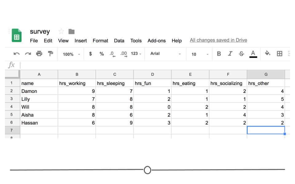
Survey Data
You'd be able to analyze these updated data using R and the googlesheets4 package!
In fact, let's have you do that right now! Click on this link to see these data!
The googlesheets4 package
The googlesheets4 package allows R users to take advantage of the Google Sheets Application Programming Interface (API). Very generally, APIs allow different applications to communicate with one another. In this case, Google has released an API that allows other software to communicate with Google Sheets and retrieve data and information directly from Google Sheets. The googlesheets4 package enables R users (you!) to easily access the Google Sheets API and retrieve your Google Sheets data.
Using this package is is the best and easiest way to analyze and edit Google Sheets data in R. In addition to the ability of pulling data, you can also edit a Google Sheet or create new sheets.
The googlesheets4 package is tidyverse-adjacent, so it requires its own installation. It also requires that you load it into R before it can be used.
Getting Started with googlesheets4
#install.packages('googlesheets4') # load package library(googlesheets4) Now, let's get to importing your survey data into R. Every time you start a new session, you need to authenticate the use of the googlesheets4 package with your Google account. This is a great feature as it ensures that you want to allow access to your Google Sheets and allows the Google Sheets API to make sure that you should have access to the files you're going to try to access.
The command gs4_auth() will open a new page in your browser that asks you which Google account you'd like to have access to. Click on the appropriate Google user to provide googlesheets4 access to the Google Sheets API.
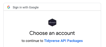
Authenticate
After you click 'ALLOW,' giving permission for the googlesheets4 package to connect to your Google account, you will likely be shown a screen where you will be asked to copy an authentication code. Copy this authentication code and paste it into R.
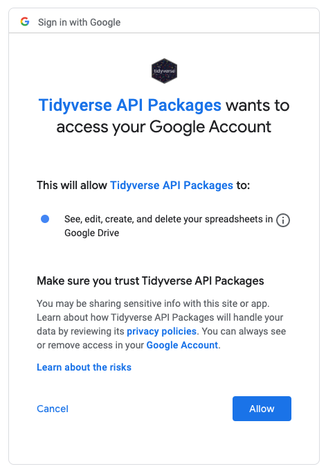
Allow
Navigating googlesheets4:gs4_find()
Once authenticated, you can use the command gs4_find() to list all your worksheets on Google Sheets as a table. Note that this will ask for authorization of the googledrive package. We will discuss more about googledrive later.
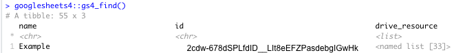
gs4_find()
Reading data in using googlesheets:gs_read()
In order to ultimately access the information a specific Google Sheet, you can use the read_sheets() function by typing in the id listed for your Google Sheet of interest when using gs4_find().
# read Google Sheet into R with id read_sheet('2cdw-678dSPLfdID__LIt8eEFZPasdebgIGwHk') # note this is a fake id You can also navigate to your own sheets or to other people's sheets using a URL. For example, paste [https://docs.google.com/spreadsheets/d/1FN7VVKzJJyifZFY5POdz_LalGTBYaC4SLB-X9vyDnbY/] in your web browser or click here. We will now read this into R using the URL:
# read Google Sheet into R with URL survey_sheet <- read_sheet('https://docs.google.com/spreadsheets/d/1FN7VVKzJJyifZFY5POdz_LalGTBYaC4SLB-X9vyDnbY/') Note that we assign the information stored in this Google Sheet to the object survey_sheet so that we can use it again shortly.
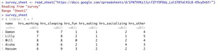
Sheet successfully read into R
Note that by default the data on the first sheet will be read into R. If you wanted the data on a particular sheet you could specify with the sheet argument, like so:
# read specific Google Sheet into R wih URL survey_sheet <- read_sheet('https://docs.google.com/spreadsheets/d/1FN7VVKzJJyifZFY5POdz_LalGTBYaC4SLB-X9vyDnbY/', sheet = 2) If the sheet was named something in particular you would use this instead of the number 2.
Here you can see that there is more data on sheet 2:
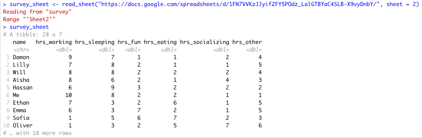
Specific Sheet successfully read into R
There are other additional (optional) arguments to read_sheet(), some are similar to those in read_csv() and read_excel(), while others are more specific to reading in Google Sheets:
-
skip = 1: will skip the first row of the Google Sheet
-
col_names= FALSE`: specifies that the first row is not column names
-
range = 'A1:G5': specifies the range of cells that we like to import is A1 to G5
-
n_max = 100: specifies the maximum number of rows that we want to import is 100
In summary, to read in data from a Google Sheet in googlesheets4, you must first know the id, the name or the URL of the Google Sheet and have access to it.
See https://googlesheets4.tidyverse.org/reference/index.html for a list of additional functions in the googlesheets4 package.
CSVs
Like Excel Spreadsheets and Google Sheets, Comma-separated values (CSV) files allow us to store tabular data; however, it does this in a much simple format. CSVs are plain-text files, which means that all the important information in the file is represented by text (where text is numbers, letters, and symbols you can type on your keyboard). This means that there are no workbooks or metadata making it difficult to open these files. CSVs are flexible files and are thus the preferred storage method for tabular data for many data scientists.
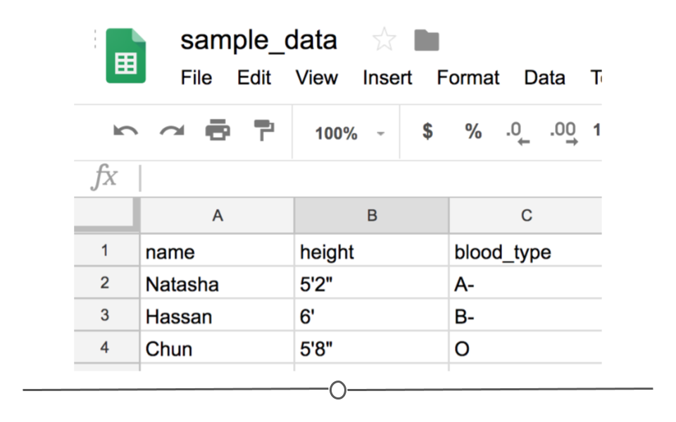
For example, consider a dataset that includes information about the heights and blood types of three individuals. You could make a table that has three columns (names, heights, and blood types) and three rows (one for each person) in Google Docs or Microsoft Word. However, there is a better way of storing this data in plain text without needing to put them in table format. CSVs are a perfect way to store these data. In the CSV format, the values of each column for each person in the data are separated by commas and each row (each person in our case) is separated by a new line. This means your data would be stored in the following format:
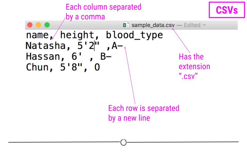
sample CSV
Notice that CSV files have a .csv extension at the end. You can see this above at the top of the file. One of the advantages of CSV files is their simplicity. Because of this, they are one of the most common file formats used to store tabular data. Additionally, because they are plain text, they are compatible with many different types of software. CSVs can be read by most programs. Specifically, for our purposes, these files can be easily read into R (or Google Sheets, or Excel), where they can be better understood by the human eye. Here you see the same CSV opened in Google Sheets, where it's more easily interpretable by the human eye:
CSV opened in Google Sheets
As with any file type, CSVs do have their limitations. Specifically, CSV files are best used for data that have a consistent number of variables across observations. In our example, there are three variables for each observation: 'name,' 'height,' and 'blood_type.' If, however, you had eye color and weight for the second observation, but not for the other rows, you'd have a different number of variables for the second observation than the other two. This type of data is not best suited for CSVs (although NA values could be used to make the data rectangular). Whenever you have information with the same number of variables across all observations, CSVs are a good bet!
Downloading CSV files
If you entered the same values used above into Google Sheets first and wanted to download this file as a CSV to read into R, you would enter the values in Google Sheets and then click on 'File' and then 'Download as' and choose 'Comma-separated values (.csv, current sheet).' The dataset that you created will be downloaded as a CSV file on your computer. Make sure you know the location of your file (if on a Chromebook, this will be in your 'Downloads' folder).
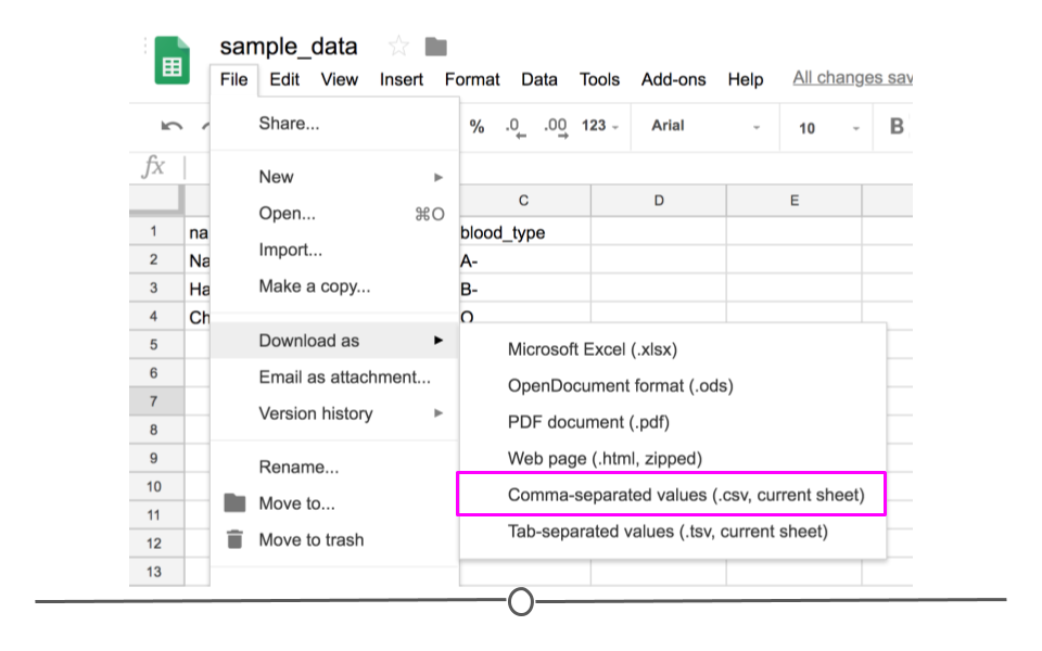
Download as CSV file
Reading CSVs into R
Now that you have a CSV file, let's discuss how to get it into R! The best way to accomplish this is using the function read_csv() from the readr package. (Note, if you haven't installed the readr package, you'll have to do that first.) Inside the parentheses of the function, write the name of the file in quotes, including the file extension (.csv). Make sure you type the exact file name. Save the imported data in a data frame called df_csv. Your data will now be imported into R environment. If you use the command head(df_csv) you will see the first several rows of your imported data frame:
## install.packages('readr') library(readr) ## read CSV into R df_csv <- read_csv('sample_data - Sheet1.csv') ## look at the object head(df_csv) 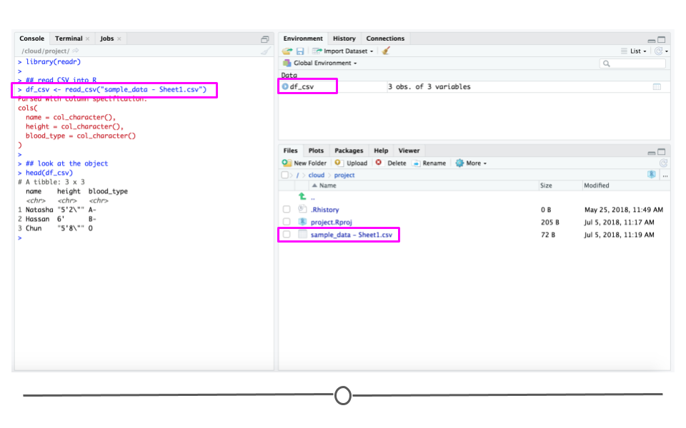
read_csv()
Above, you see the simplest way to import a CSV file. However, as with many functions, there are other arguments that you can set to specify how to import your specific CSV file, a few of which are listed below. However, as usual, to see all the arguments for this function, use ?read_csv within R.
-
col_names = FALSEto specify that the first row does NOT contain column names. -
skip = 2will skip the first 2 rows. You can set the number to any number you want. This is helpful if there is additional information in the first few rows of your data frame that are not actually part of the table. -
n_max = 100will only read in the first 100 rows. You can set the number to any number you want. This is helpful if you're not sure how big a file is and just want to see part of it.
By default, read_csv() converts blank cells to missing data (NA).
We have introduced the function read_csv here and recommend that you use it, as it is the simplest and fastest way to read CSV files into R. However, we note that there is a function read.csv() which is available by default in R. You will likely see this function in others' code, so we just want to make sure you're aware of it.
TSVs
Another common form of data is text files that usually come in the form of TXT or TSV file formats. Like CSVs, text files are simple, plain-text files; however, rather than columns being separated by commas, they are separated by tabs (represented by ' in plain-text). Like CSVs, they don't allow text formatting (i.e. text colors in cells) and are able to be opened on many different software platforms. This makes them good candidates for storing data.
Reading TSVs into R
The process for reading these files into R is similar to what you've seen so far. We'll again use the readr package, but we'll instead use the read_tsv() function.
## read TSV into R df_tsv <- read_tsv('sample_data - Sheet1.tsv') ## look at the object head(df_tsv) Delimited Files
Sometimes, tab-separated files are saved with the .txt file extension. TXT files can store tabular data, but they can also store simple text. Thus, while TSV is the more appropriate extension for tabular data that are tab-separated, you'll often run into tabular data that individuals have saved as a TXT file. In these cases, you'll want to use the more generic read_delim() function from readr.
Google Sheets does not allow tab-separated files to be downloaded with the .txt file extension (since .tsv is more appropriate); however, if you were to have a file 'sample_data.txt' uploaded into R, you could use the following code to read it into your R Environment, where ' specifies that the file is tab-delimited.
Reading Delimited Files into R
## read TXT into R df_txt <- read_delim('sample_data.txt', delim = ' ') ## look at the object head(df_txt) This function allows you to specify how the file you're reading is in delimited. This means, rather than R knowing by default whether or not the data are comma- or tab- separated, you'll have to specify it within the argument delim in the function.
The read_delim() function is a more generic version of read_csv(). What this means is that you could use read_delim() to read in a CSV file. You would just need to specify that the file was comma-delimited if you were to use that function.
Exporting Data from R
The last topic of this lesson is about how to export data from R. So far we learned about reading data into R. However, sometimes you would like to share your data with others and need to export your data from R to some format that your collaborators can see.
As discussed above, CSV format is a good candidate because of its simplicity and compatibility. Let's say you have a data frame in the R environment that you would like to export as a CSV. To do so, you could use write_csv() from the readr package.
Since we've already created a data frame named df_csv, we can export it to a CSV file using the following code. After typing this command, a new CSV file called my_csv_file.csv will appear in the Files section of RStudio (if you are using it).
write_csv(df_csv, path = 'my_csv_file.csv') You could similarly save your data as a TSV file using the function write_tsv() function.
We'll finally note that there are default R functions write.csv() and write.table() that accomplish similar goals. You may see these in others' code; however, we recommend sticking to the intuitive and quick readr functions discussed in this lesson.
JSON
All of the file formats we've discussed so far (tibbles, CSVs, Excel Spreadsheets, and Google Sheets) are various ways to store what is known as tabular data, data where information is stored in rows and columns. To review, when data are stored in a tidy format, variables are stored in columns and each observation is stored in a different row. The values for each observation is stored in its respective cell. These rules for tabular data help define the structure of the file. Storing information in rows and columns, however, is not the only way to store data.
Alternatively, JSON (JavaScript Object Notation) data are nested and hierarchical. JSON is a very commonly-used text-based way to send information between a browser and a server. It is easy for humans to read and to write. JSON data adhere to certain rules in how they are structured. For simplicity, JSON format requires objects to be comprised of key-value pairs. For example, in the case of: {'Name': 'Isabela'}, 'Name' would be a key, 'Isabela' would be a value, and together they would be a key-value pair. Let's take a look at how JSON data looks in R.This means that key-pairs can be organized into different levels (hierarchical) with some levels of information being stored within other levels (nested).
Using a snippet of JSON data here, we see a portion of JSON data from Yelp looking at the attributes of a restaurant. Within attributes, there are four nested categories: Take-out, Wi-Fi, Drive-Thru, and Good For. In the hierarchy, attributes is at the top, while these four categories are within attributes. Within one of these attributes Good For, we see another level within the hierarchy. In this third level we see a number of other categories nested within Good For. This should give you a slightly better idea of how JSON data are structured.
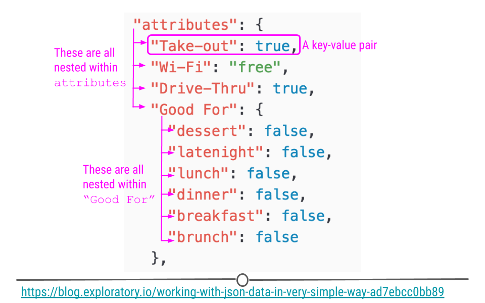
JSON data are hierarchical and nested
To get a sense of what JSON data look like in R, take a peak at this minimal example:
## generate a JSON object json <- '[ {'Name' : 'Woody', 'Age' : 40, 'Occupation' : 'Sherriff'}, {'Name' : 'Buzz Lightyear', 'Age' : 34, 'Occupation' : 'Space Ranger'}, {'Name' : 'Andy', 'Occupation' : 'Toy Owner'} ]' ## take a look json ## [1] '[
{'Name' : 'Woody', 'Age' : 40, 'Occupation' : 'Sherriff'},
{'Name' : 'Buzz Lightyear', 'Age' : 34, 'Occupation' : 'Space Ranger'},
{'Name' : 'Andy', 'Occupation' : 'Toy Owner'}
]' Here, we've stored information about Toy Story characters, their age, and their occupation in an object called json.
In this format, we cannot easily work with the data within R; however, the jsonlite package can help us. Using the defaults of the function fromJSON(), jsonlite will take the data from JSON array format and helpfully return a data frame.
#install.packages('jsonlite') library(jsonlite) ## take JSON object and covert to a data frame mydf <- fromJSON(json) ## take a look mydf ## Name Age Occupation ## 1 Woody 40 Sherriff ## 2 Buzz Lightyear 34 Space Ranger ## 3 Andy NA Toy Owner 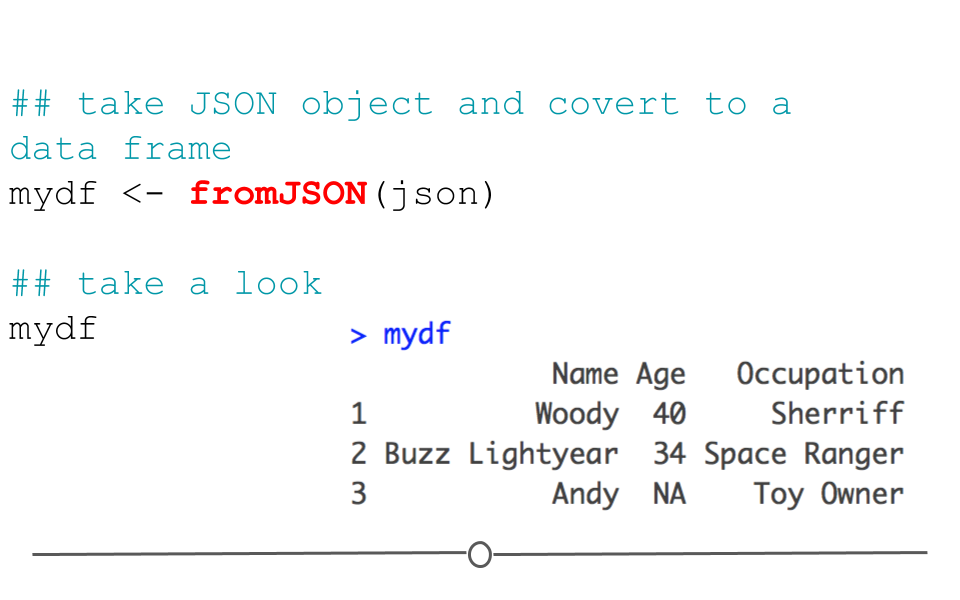
fromJSON()
Data frames can also be returned to their original JSON format using the function: toJSON().
## take JSON object and convert to a data frame json <- toJSON(mydf) json 


No comments:
Post a Comment